Methodology · Ski Resort Trail Maps & GPS Data

Methodology

How the painted Shiga Kogen trail map is georeferenced: data sources, the six-step workflow, and a specification detailed enough to rebuild it.

← Back to the overview

Data sources

SourceWhat it providesSize used here
Shiga Kogen Lift Association trail mapThe painted panorama: runs, lifts, station markers, area labels3,000 × 961 px, upscaled to 6,000 × 1,922
GSI (Geospatial Information Authority of Japan) DEM1A1 m elevation model from airborne LiDAR: the 3D terrain everything is projected from2,048 tiles, 148 MB
GSI DEM5A5 m elevation, to fill gaps in the 1 m data153 tiles
GSI seamless orthophotoAerial photograph (Fig. 2 on the overview page), about 0.3 m per pixel8,001 tiles, 182 MB
GSI survey benchmarksSurveyed summit heights for the 9 peaks used as control points14 peaks
OpenStreetMapLifts, ski runs (with difficulty), ski-area outlines and named peaks52 lifts, 237 runs, 18 areas
Hand-made tablesLift-end ↔ painted-marker pairing, painted label positions, lift-number ↔ OSM lift, 5 station corrections79 lift ends, 47 lift numbers
Phone GPSMy own tracks: position and time at 1 Hz, resampled to 5 s6 days, 45 hours, 180 km, 33,365 m descended

Workflow

1

Control points

The painting marks every lift’s bottom and top station with a black dot or triangle. Those, plus labelled summits, are the features that can be located exactly in both the image and map data.

Detect
Dark ink with the label text removed, opened and filtered by size: 86 candidate markers.
Match
Paired by hand to OpenStreetMap lift ends using the painted lift numbers: 79 lift ends (69 from detected markers, 10 read off the image by hand) plus 9 peaks from the painted ▲, 88 pairs of ground point (x, y, z) ↔ pixel (u, v). Ground heights come from the GSI (Geospatial Information Authority of Japan) 1 m DEM.
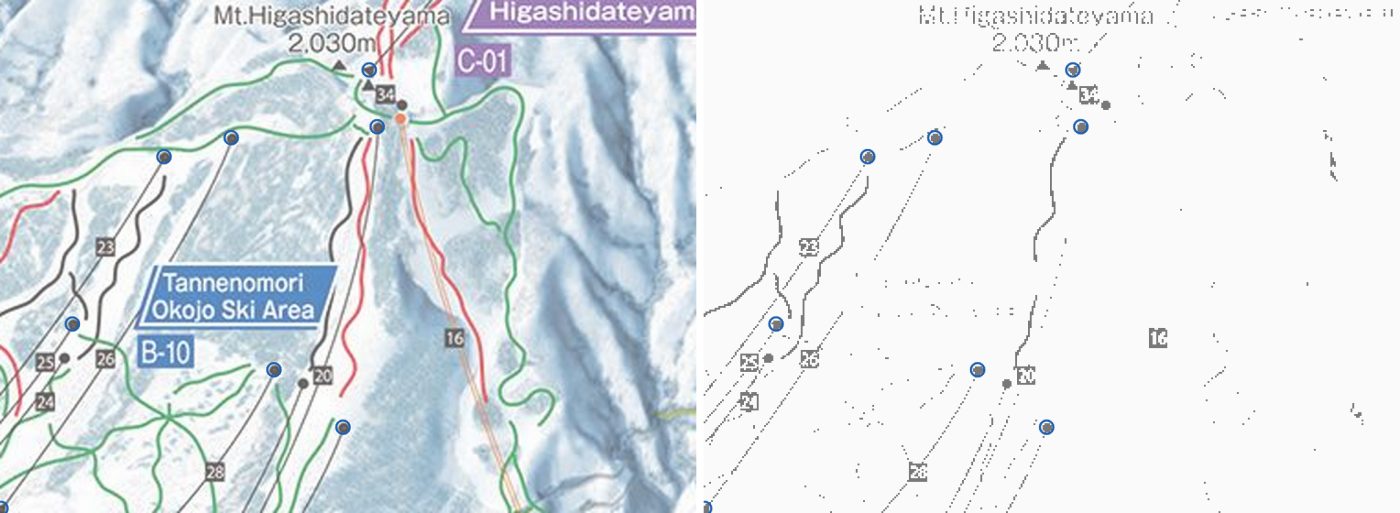
Painting crop beside its dark-ink mask with detected lift terminals circled
Fig. M1 Around Mt Higashidateyama. Left: the painting. Right: the dark-ink mask. Circles are detected terminals; blue ones are used as control points.
2

Camera fit

Treat the painting as a photo: find the single pinhole camera that best projects the 88 ground points onto their painted pixels. One extra parameter scales every height before projection, because painters stretch relief to make slopes readable. Because the model is a 3D projection, it accounts for terrain height, and the same camera gives the visibility test used for the coverage maps.

# 10 parameters; scene axes x east, y up, z south (metres)
def project(p, P):
    cx, cy, cz, yaw, pitch, roll, f, u0, v0, ex = p
    d = (P * [1, ex, 1] - [cx, cy, cz]) @ rot(yaw, pitch, roll).T
    return u0 + f * d[:, 0] / d[:, 2], v0 - f * d[:, 1] / d[:, 2]
Solve
Robust bounded least squares, started from a coarse multi-start fit on peaks and lift-number labels.
Result
Viewpoint 9.7 km west of the resort centre, heading 1.8° north of east, pitched 10.2° down, roll −4.6°, focal length 2,169 px, vertical exaggeration 2.50×.
Error
Median 66 px, 90th percentile 216 px (on the 3,000 px wide image). Too large to place tracks with.
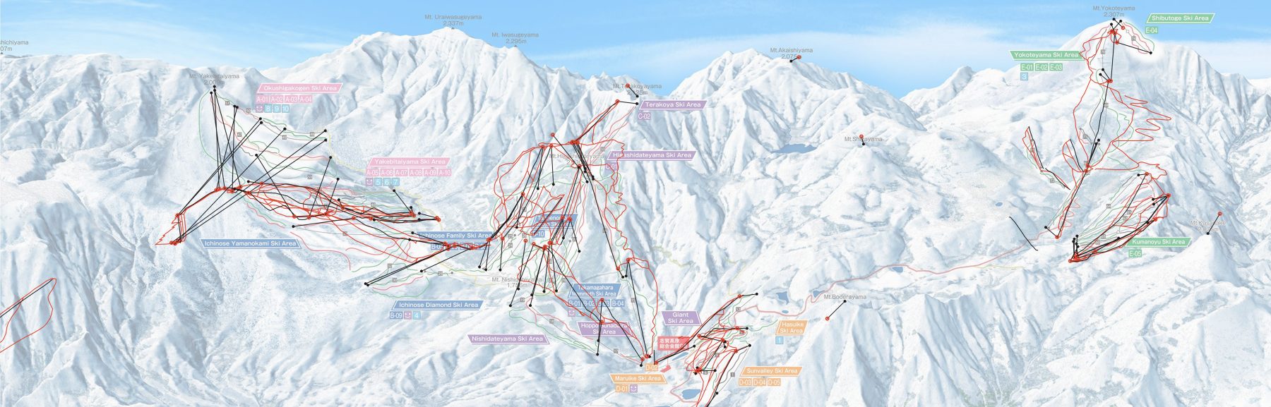
Whole panorama with OSM runs projected by the camera only and control-point residuals
Fig. M2 OSM runs through the camera only . Each black line joins a control point’s predicted position to where it is painted . The misses are largest in the far west (Okushiga, Yakebitai), which the artist pulled closer.
3

Thin-plate spline on the residuals

The camera’s leftover errors (painted pixel minus predicted pixel) are smooth across the landscape: whole areas were shifted or compressed by the artist. A thin-plate spline interpolates that 2D offset over ground position, and is added to the camera projection.

uv(P) = camera(P) + TPS(P.x, P.z)
# scipy.interpolate.RBFInterpolator(kernel="thin_plate_spline"), positions in km,
# smoothing = 0.03 / (w_i · mean(w))

Interpolating over the ground rather than the image leaves the camera in charge of height; the spline only shifts points within the image plane. Light smoothing tolerates small disagreements between a painted marker and its OSM position.

Error
Leave-one-out (predict each control point from the other 87; camera not refit): median 25 px, 90th percentile 89 px. This is the expected error away from the control points.
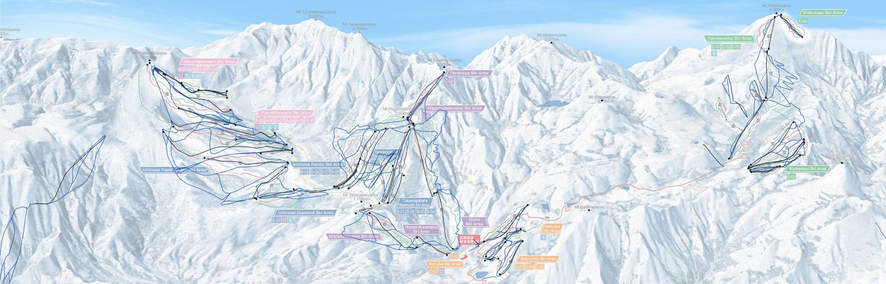
Whole panorama with OSM runs projected by camera plus spline, now following the painted runs
Fig. M3 The same OSM runs through camera + spline , with lifts in black. Lift ends land on their markers, and runs follow the painted lines. Switch the interactive map on the overview page to “Final mapping” to see the ground grid morph from the camera-only fit to the full mapping.
4

Chamfer refinement against the painted runs

The painted runs provide many more constraints than the 88 points. A second, low-frequency correction moves the projected OSM runs onto the painted line of the same colour.

Target
Masks of the green, red and black runs and the lift cables (from the ink unmixing in the specification), each turned into a distance field.
Field
Gaussian RBF nodes every 550 m over the ski terrain (114 nodes × 2 offsets). OSM runs and unpinned lifts densified to 12 m, then filtered: 7,161 run samples and 170 lift samples kept.
Solve
Minimise each sample’s distance to its class’s painted line, capped at 14 px so runs the artist never drew are ignored. Penalties keep the control points in place and the offsets small.
Result
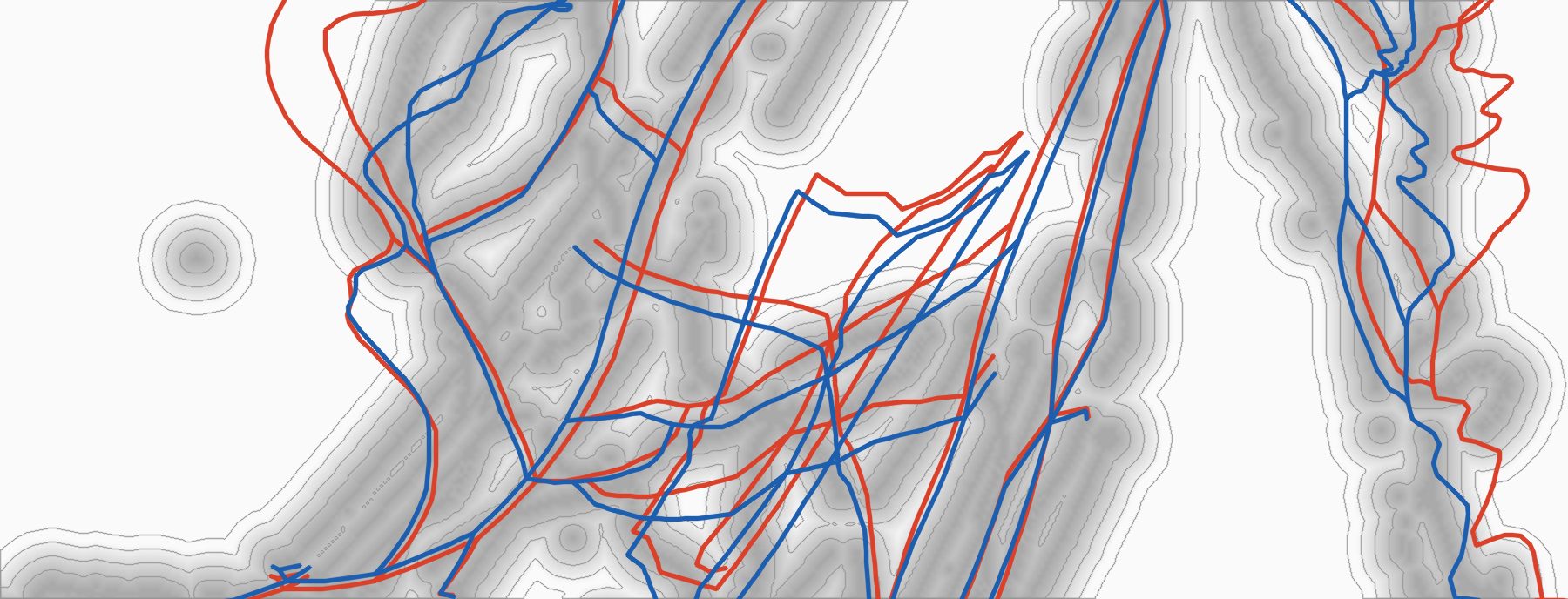
Median distance to the painted line 8.5 → 3.5 px; samples within 3 px 22% → 46%. Control points end up a median 12 px (90th percentile 26 px) from their painted positions, up from 6 px after the spline alone.
Distance field around painted runs with OSM runs before and after refinement
Fig. M4 Distance to the nearest painted run (darker grey is closer; rings every 4 px), Ichinose to Takamagahara. OSM runs before and after refinement.
5

Bake a lookup grid

The fitted model needs the DEM, the camera, 88 spline centres and 114 refinement nodes, which is too heavy to hand to a web page. For use elsewhere the model is evaluated once on a regular latitude/longitude grid, and a client interpolates between nodes. The overview page’s interactive map doesn’t use it, since its tracks are projected offline with the full model, but the grid is the portable form of the result.

Grid
40 m spacing, 182 columns × 360 rows, covering every run and lift on the painting plus 800 m. Each node stores its pixel (u, v) × 10 as integers: 709 KB of JSON.
Accuracy
Bilinear lookup vs the full model: median 0.42 px, 99th percentile 3.0 px. Ground height is baked in, so the noisy GPS altitude is never needed.
const nx = 182, ny = 360;                 // columns, rows; row 0 is the northernmost, latitudes descending
function toPixel(lat, lon) {              // bilinear between the 4 surrounding nodes
  const fx = (lon - G.west) / G.dlon, fy = (G.north - lat) / G.dlat;
  const i = Math.floor(fx), j = Math.floor(fy), a = fx - i, b = fy - j;
  const k = j * nx + i;                   // U and V are flat row-major arrays
  const at = A => A[k]*(1-a)*(1-b) + A[k+1]*a*(1-b) + A[k+nx]*(1-a)*b + A[k+nx+1]*a*b;
  return [at(U) / 10, at(V) / 10];
}
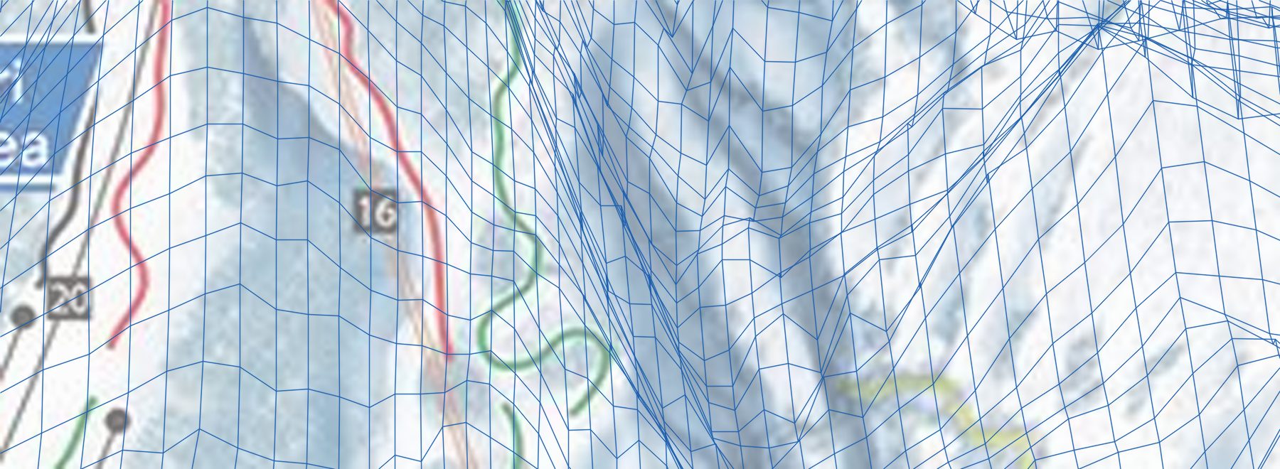
Every 40 m grid node projected onto a crop of the painting near lift 16
Fig. M5 The grid at full density by the Higashidateyama gondola (lift 16). Squares on the ground become stretched quadrilaterals. Lines bunch up where the slope faces away from the viewer and occupies little of the painting.
6

Tracks and rendering

  • Phone GPS at 1 Hz is smoothed and labelled run / lift / stop (rules in the specification). Each fix is projected through the full model with its height from the DEM, then resampled to 5 s.
  • Lift rides are not projected directly. The painted lift lines are straight but displaced for clarity, so a fix 40% of the way along the real lift is drawn 40% of the way along the painted one.
  • Packed as Int16 u, Int16 v, Uint8 state, Uint8 km/h: 6 bytes per sample.
  • The browser only draws, with Canvas 2D. Tracks get a white casing so they read against the painted runs.

Specification

Enough detail to rebuild the pipeline. Library calls are Python (NumPy, SciPy, OpenCV) unless noted. Long entries fold open.

Frames
Ground: local metric frame in metres, x east, z south, y height above 886 m. Image: u right, v down, in pixels of the 3,000 × 961 source; the page doubles them for its 6,000 px copy.
Scene origin
Bounding box S 36.656, N 36.794, W 138.468, E 138.554. Web Mercator at zoom 17: px = (lon + 180)/360 · 256 · 217, py = (1 − asinh(tan lat)/π)/2 · 256 · 217. The grid origin is the box’s north-west corner, (X0, Y0) = (29,683,369, 13,084,403), and the grid is W × H = 8,016 × 16,048 px. Then x = (px − X0 − W/2)·m, z = (py − Y0 − H/2)·m, with one constant m = 0.95727 m/px (the mid-latitude value).
DEM
GSI 1 m tiles: URL, decoding, voids, subsampling

Tiles: https://cyberjapandata.gsi.go.jp/xyz/dem1a_png/17/{x}/{y}.png, mosaicked onto the grid above. Decode n = R·65536 + G·256 + B; height is 0.01·n m if n < 223, nodata if n = 223, otherwise 0.01·(n − 224) m. Voids are filled bilinearly from the 5 m tiles (dem5a_png/15), then from the nearest valid cell. Scene height is y = h − 886.

The fits, the visibility test, the grid and the track projection all read the grid subsampled every 8 px (h[::8, ::8], 1,002 × 2,006), bilinear, with cell k centred at (k + ½)·8 px.

OSM
Overpass queries, lift and piste classes, peaks

Overpass, bbox 36.656,138.468,36.794,138.554 (S, W, N, E). Runs and lifts: [out:json][timeout:180];(way["aerialway"](bbox);way["piste:type"](bbox););out geom tags; (the piste and lift part of fetch_osm.sh, which also fetches buildings and roads). Lift geometry with pylon and station nodes: (way["aerialway"](bbox);way["disused:aerialway"](bbox);node["aerialway"](bbox);)->.a;(.a;.a>;);out body;.

Lifts: aerialway = chair_lift or gondola, 52 lines (46 chairlifts, 6 gondolas), each oriented bottom → top by DEM height. Pistes: piste:type = downhill or connection; difficulty easy or novice → green, intermediate → red, advanced, expert, freeride, extreme and unrated → black (a connection without a grade counts as green). Lifts form the cable class. Peaks: named natural=peak nodes, position from OSM, elevation from the nearest GSI survey benchmark within 200 m, else the ele tag; the fit uses y = ele − 886.

Hand data
Control-point pairing, painted labels, peak names, lift overrides

These are hand-made, not derivable from public data. ctrl.json: lift number → [bottom, top], each end a marker index into markers.json or a literal [u, v] in source pixels; 40 lifts, 79 ends, 10 of them literal. labels.json: painted label positions (peak name lines and summit triangles, lift numbers). The lift number ↔ OSM way table lives in each lift’s English name (lift #16). Five OSM lift ways carry hand-corrected station positions (overrides.json, keyed by way id: corrected bottom and top lon/lat, the way’s other points keep their fractions along the line).

Peak names, painted label → OSM name: Yakebitaiyama → Mt Yakebitai, Terakoyayama → Terakoya Peak, Higashidateyama → Mt Higashidate, Akaishiyama → Mt Akaishi, Shigayama → Mt Shiga, Yokoteyama → Mt Yokote, Nishidateyama → Mt Nishidate, Boderayama → Mt Bodera, Kasadake → Mt Kasagatake.

An automatic pairing should be possible but I haven’t tried it: run the coarse camera fit, project each OSM lift end, take the nearest unused marker within about 80 px, and call the end with the lower DEM height the bottom.

Ink unmixing
Palette, terrain estimate, per-colour coverage (masks for step 4)

Palette (RGB): green (18, 140, 62), red (212, 22, 34), black (12, 10, 10), yellow (214, 216, 70), road (205, 88, 96), gondola (232, 150, 100), dot (242, 104, 30), gondola core (246, 214, 182). Candidates: pixels with saturation > 45 (not blue) or value < 55, plus thin dark components (black-hat with a 7 px ellipse > 30, components of at least 25 px² and 12 px extent), minus the hand-annotated label boxes.

Provisional terrain T = cv2.inpaint(src, dilate(candidates, 5×5 ellipse) ∪ label ink, 4, INPAINT_TELEA). Per palette colour C, a = clip((P − T)·(C − T)/|C − T|², 0, 1); each pixel takes the colour with the smallest residual |P − (a·C + (1 − a)·T)|, and a < 0.12 is rejected. Black keeps only components of a > 0.2 that contain a > 0.85. The gondola core counts only within 7 px of gondola edge ink. Masks are a > 100/255.

1 · Pairs
Terminal markers: grey < 70 and HSV value < 90, label ink masked out (dilated 5 × 5), cv2.morphologyEx open with a 3 × 3 ellipse, components of 8–120 px² with bbox ≤ 14 px: 86 markers (fill fraction > 0.68 = dot, else triangle). Each lift end is paired by hand with a marker (or a literal pixel) via the painted lift number; bottom = the end with the lower DEM height. Summits: painted ▲ ↔ OSM natural=peak by name. Result: 88 pairs (Xi, ui): 79 lift ends (69 from detected markers, 10 read off the image by hand; weight 1.0) and 9 peaks (weight 0.6).
2 · Camera
Parameters p = (cx, cy, cz, yaw, pitch, roll, f, u0, v0, e); c is in exaggerated space and the principal point is free (it ends up off the image). X' = (x, e·y, z), d = R(X' − c) = (dr, du, dfwd), u = u0 + f·dr/dfwd, v = v0 − f·du/dfwd; depth is dfwd. Minimise Σ ρ(wi·(π(Xi) − ui)) with scipy.optimize.least_squares, loss="soft_l1", f_scale=25.
Rotation
fwd = (cos yaw·cos pitch, sin pitch, sin yaw·cos pitch), right = (−sin yaw, 0, cos yaw), up = right × fwd. Roll: r = right·cos roll + up·sin roll, u' = up·cos roll − right·sin roll. R has rows [r; u'; fwd]. At yaw 0 forward is +x (east) and positive yaw turns south. Fitted p = (−9738.8, 6458.1, 1666.2, −0.03228, −0.17748, −0.08043, 2169.1, 1686.5, −36.57, 2.5004) (metres, radians, pixels).
Camera solve
Bounds, scaling and the coarse fit that starts it

Main fit bounds: cx [−80, −3] km, cy [0.5, 60] km, cz ±20 km, yaw ±1.2, pitch [−0.8, 0.3], roll ±0.3, f [300, 60,000], u0 [−2,000, 5,000], v0 [−4,000, 3,000], e [0.8, 4]. x_scale = (1000, 500, 1000, .1, .1, .05, 500, 200, 200, .3), max_nfev = 5000. The start is the coarse fit with e = 1.5, clipped to the bounds.

Coarse fit (fit0.py, no e): summits (weight 1.0) plus painted lift-number labels taken as lift midpoints (weight 0.35), soft_l1 with f_scale = 20, max_nfev = 4000, bounds cx [−60, −3] km, cy [0.5, 30] km, pitch [−0.8, 0.2], f [300, 20,000], u0 [500, 2,500], v0 ±3,000. Multi-start over cx ∈ {−9, −14, −20} km × yaw ∈ {−0.3, 0, 0.3}, each from (cx, 3500, 800, yaw, −0.15, 0, 2500, 1500, 300); keep the lowest cost.

3 · Spline
Residuals ri = ui − π(Xi) fitted over ground position with RBFInterpolator((x, z)/1000, r, kernel="thin_plate_spline", smoothing=0.03/(wi·mean(w))), positions in km. M0(X) = π(X) + TPS(x, z).
4 · Chamfer
Distance fields Dk = cv2.distanceTransform(~maskk, DIST_L2, 5) in source pixels for green, red and black runs and for cables (black ∪ gondola ∪ gondola core), sampled bilinearly and clamped at the border. Samples: OSM pistes (easy and novice → green, intermediate → red, the rest → black) and the 13 lifts that are not pinned (a lift is pinned when both its ends are control points: 39 of 52), densified to 12 m horizontally; kept if M0 puts them inside the frame (5 px margin) and D < 40 px: 7,161 run samples and 170 lift samples. Nodes: a 550 m grid from min − 550 to max + 550 over the kept samples, kept if within 550 m of every 7th sample: 114 nodes. Correction δ(x, z) = Σj exp(−|g − gj|² / 2σ²)·oj, σ = 500 m, oj in source pixels. Residual vector: min(Dk(M0 + δ), 14) (lift samples × 1.5), 1.2·δ(Xi) at the control points, 1.0·o; the gradient is 0 where D ≥ 14. least_squares(loss="soft_l1", f_scale=3, max_nfev=200) with an analytic Jacobian from the distance-field gradients, run three times, each a warm restart from the last solution (no blur schedule). M = M0 + δ.
Visibility
Project every DEM cell through the camera and keep the minimum depth per 4 × 4 px bucket (source pixels, with a 200 px margin). A point is visible if it is in front of the camera and its depth ≤ 1.015 × bucket + 60 m. Used for the ski-area fills and the coverage maps, not for the lookup.
5 · Grid
A portable copy of M. Nodes every 40 m (dlat = 40/111320, dlon = dlat/cos φ) over all runs and lifts in frame + 800 m: 182 columns × 360 rows, latitudes descending. At each node, X = (x, DEM(x, z), z), stored as round(10·M(X)), row-major from the north-west. JSON: {grid: {west, north, dlon, dlat, nx, ny}, u: [...], v: [...]}. Bilinear lookup against the full model: median 0.42 px, 99th percentile 3.0 px.
6 · Runtime
The browser only draws. Tracks are projected offline with the full model M: each fix becomes X = (x, DEM(x, z), z) and uv = M(X), so GPS altitude is ignored. Tracks are labelled run / lift / stop, sampled every 5 s (the first fix at or after each time) and packed. Tracks starting at or after 17:00 are dropped.
GPS labels
Cleaning, smoothing, and the run / lift / stop rules

1 Hz fixes. Drop fixes that imply > 35 m/s from the last good one; split into segments at gaps > 8 s or > 60 m. Per segment a constant-velocity Kalman filter with an RTS smoother; heights are re-read from the DEM along the smoothed path. Speed is measured along the slope: hypot(horizontal speed, vertical rate over ~5 s).

Run: speed > 2.2 m/s and vertical rate < 0.4 m/s (rests of up to 25 fixes and run blips of up to 8 fixes are absorbed into the surrounding state). Lift: per lift line, fixes within 35 m of the line (plus half the cable gauge) form visits; a visit is a ride if it climbs at least max(80 m, 35% of the line) along the line at 0.25–1.3 × the line’s speed, the ground under it rises at least 30% of the lift’s own vertical over that stretch, and the fixes follow a monotone fit (median residual ≤ 12 m). Everything else is stop.

Lift snap
A ride fix at ground position P on a lift with real ends A (bottom) and B (top): f = clip((P − A)·(B − A)/|B − A|², 0, 1), uv = a + f·(b − a), where a and b are the painted ends: the control-point pixels where the end is pinned, else the model projection.
Packing
Planar arrays Int16 u, Int16 v (6,000 px space), Uint8 state (0 stop, 1 lift, 2 run) and Uint8 km/h, one entry per 5 s step.

What the painting covers and how much it distorts

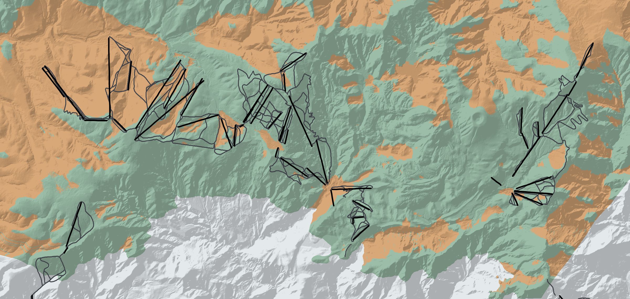
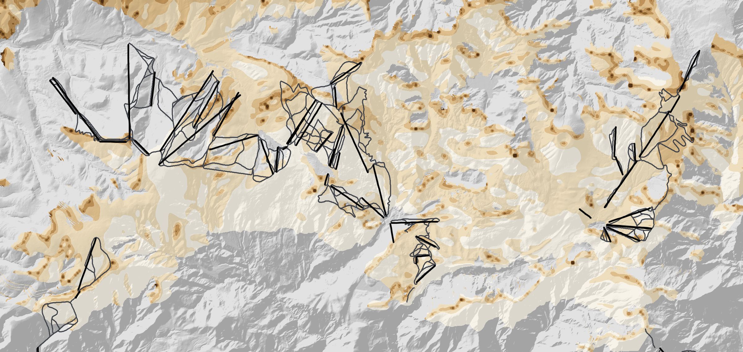
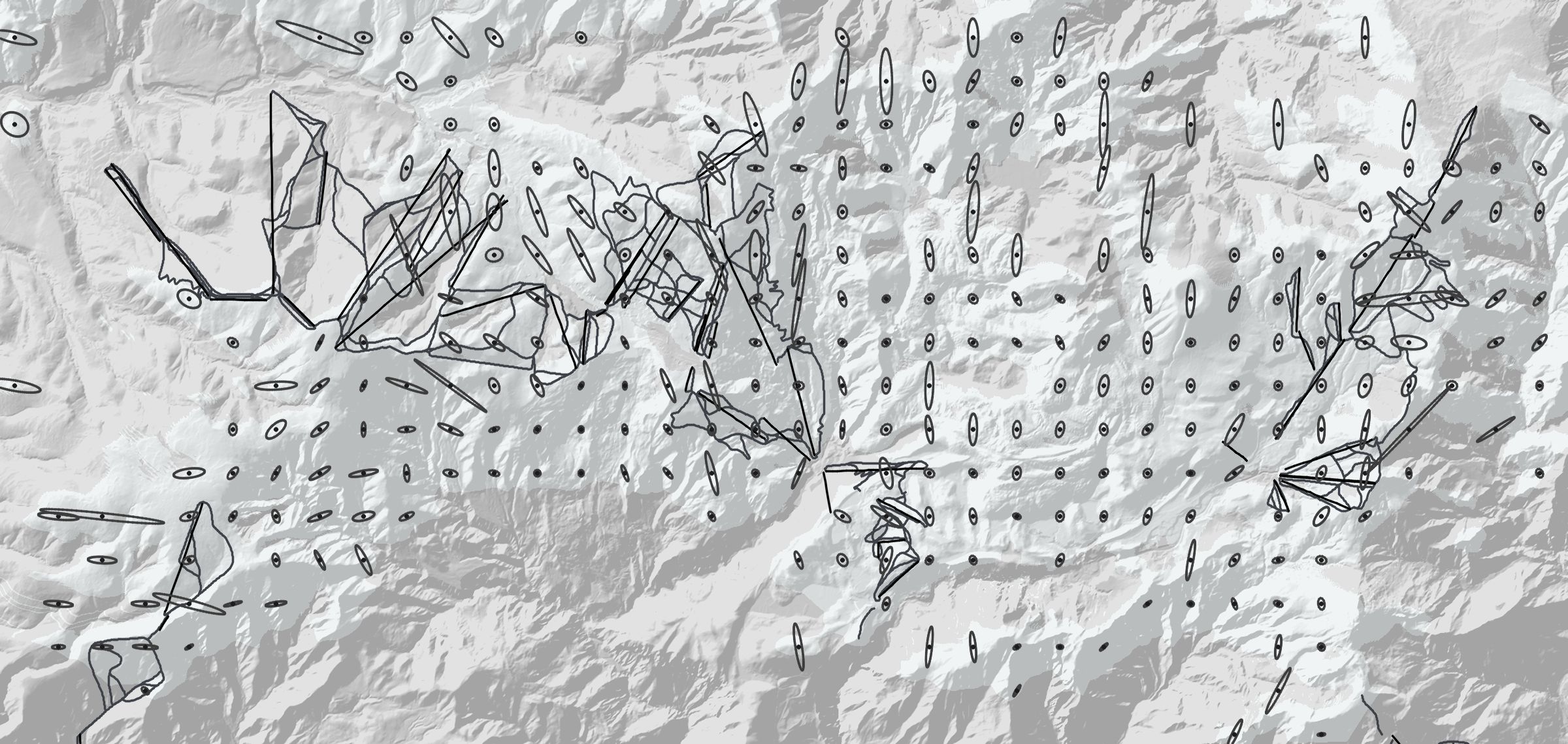
The lookup gives, for every ground point, where it lands in the painting. That shows which terrain the painting covers at all and how much of it is stretched or squeezed. Fig. M6 draws this on a map with north to the left, as in Fig. 2 on the overview page, so east is up and the painter looks toward the top. It covers 98 km² of terrain; thin grey lines are OpenStreetMap runs and black lines are lifts.

Show
N
Fig. M6 The painting on the ground, north to the left. Coverage: what the painting shows, hides behind a ridge, or leaves out. Scale: ground metres per painted pixel (3,000 px source), painted ground only. Stretch: the ground footprint of a fixed circle in the painting, one per 400 m. Drag to pan; click the map, then scroll or pinch to zoom.

Coverage. About 52% of the terrain is painted, 30% is hidden behind ridges from the painter’s viewpoint and 18% lies outside the frame. The runs fare better than the terrain as a whole: 71% of the sampled run length is painted, 21% is hidden and 8% is outside; for lifts the figures are 71%, 27% and 2%. Hidden ground is what the artist had to leave out or draw on the ridge line, so tracks there cannot be placed accurately.

Scale. One painted pixel covers a median 5.7 m of ground (linear, geometric mean of the two directions); 83% of painted ground is under 10 m per pixel and the 95th percentile is 18 m. The coarse areas (dark, 40 m per pixel and more, under 1% of painted ground) are slopes turned away from the viewer and isolated summits seen edge-on.

Stretch. Each ellipse is the ground area covered by a circle of 9 painted pixels; a circle would mean no distortion. The median ellipse is 2.5 times longer than wide, 41% are more than 3 times, and 9% more than 10 times. Where they point along a ridge, the painting squeezes that ridge into a few pixels, and a GPS track there moves fast across the painting for a small ground distance.

Known issues